IB Physics A.1 Kinematics | Lesson 2 | SL/HL

Uniformly Accelerated Motion and SUVAT

Guiding question: When is one constant-acceleration model justified, and which equation exposes the unknown most directly?

Learning Objectives and Success Criteria

Understand

instantaneous velocity and acceleration
sign reasoning
uniform-acceleration assumptions

Apply

derive and select SUVAT equations
declare a sign convention
test a model against evidence

Starter | Retrieve Motion Quantities

A shuttle moves along a straight corridor. Take east as positive. From $t = 0$ to $4.0 s$ , its velocity is $+ 2.0 m s^{- 1}$ . From $t = 4.0 s$ to $7.0 s$ , its velocity is $- 1.0 m s^{- 1}$ .

The velocity-time representation consists of two horizontal segments: $+ 2.0 m s^{- 1}$ for $4.0 s$ , followed by $- 1.0 m s^{- 1}$ for $3.0 s$ .

(a) Determine the total distance travelled and the displacement during the $7.0 s$ interval.
(b) State whether one constant-velocity model is valid for the complete $7.0 s$ interval.
(c) Use signed area under the velocity-time representation to determine the displacement.

Reveal Q1 (1)

Distance $= 11 m$ ; displacement $= + 5.0 m$ (east).

The eastward distance is $(2.0) (4.0) = 8.0 m$ . The westward distance is $(1.0) (3.0) = 3.0 m$ , so total distance is $8.0 + 3.0 = 11 m$ . The signed displacement is $+ 8.0 - 3.0 = + 5.0 m$ .

Reveal Q1 (2)

No.

Velocity changes from $+ 2.0 m s^{- 1}$ to $- 1.0 m s^{- 1}$ at $4.0 s$ . One constant-velocity model cannot describe both intervals, although each horizontal segment can be modelled separately.

Reveal Q1 (3)

$+ 5.0 m$ .

Signed area is $(+ 2.0) (4.0) + (- 1.0) (3.0) = + 8.0 - 3.0 = + 5.0 m$ . The negative rectangle subtracts from displacement but still contributes positively to distance.

Instantaneous Velocity Is a Local Gradient

Finite interval

Average velocity is the average rate of change of position.

On a position-time graph, it is represented by the gradient of the chord joining the two interval endpoints.

\bar{v} = \frac{Δ x}{Δ t}

A chord across a finite interval gives average velocity; it is not the instantaneous value unless the graph is locally straight.

One instant

On an ideal mathematical graph, the tangent gradient at one point gives instantaneous velocity.

Measured data uses a tangent or shrinking interval to estimate instantaneous velocity.

As the interval narrows, the chord approaches the tangent.

Instantaneous Velocity Check | Chord or Tangent?

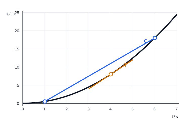
Position-time graph with a chord from 1 to 6 seconds and a tangent at 4 seconds

Figure 1 | One motion model, two gradients.

Figure 1 is a project-created position-time graph for a delivery robot whose position is defined by $x (t) = 0.50 t^{2}$ , with $x$ in metres and $t$ in seconds. Line C is a chord joining two points on the curve. Line T is tangent to the curve at $t = 4.0 s$ .

For calculation, line C passes through $(1.0 s, 0.50 m)$ and $(6.0 s, 18.0 m)$ . Line T touches the curve at $(4.0 s, 8.0 m)$ and passes through $(3.0 s, 4.0 m)$ and $(5.0 s, 12.0 m)$ .

(a) Identify which line, C or T, is used to estimate the instantaneous velocity at $t = 4.0 s$ .
(b) Determine (i) the average velocity from $1.0 s$ to $6.0 s$ and (ii) the instantaneous velocity at $4.0 s$ .

Reveal Q1 (1)

Line T.

Instantaneous velocity is estimated by the gradient of the tangent at the specified instant. Line T touches the curve locally at $t = 4.0 s$ .

Reveal Q1 (2)

(i) $3.5 m s^{- 1}$ ; (ii) $4.0 m s^{- 1}$ .

The chord gradient is $\frac{18.0 - 0.50}{6.0 - 1.0} = 3.5 m s^{- 1}$ , which is the finite-interval average velocity. The tangent gradient is $\frac{12.0 - 4.0}{5.0 - 3.0} = 4.0 m s^{- 1}$ . This agrees with the local gradient of $x (t) = 0.50 t^{2}$ at $t = 4.0 s$ , so it is the instantaneous velocity.

Acceleration Measures How Velocity Changes

Average acceleration

a_{avg} = \frac{Δ v}{Δ t}

Use the full stated interval.

Instantaneous acceleration

The local gradient of a velocity-time graph.

Negative acceleration records direction; it does not automatically mean the object is slowing down.

Compare the Signs of Velocity and Acceleration

v +, a +

speeding up

v +, a −

slowing down

v −, a −

speeding up

v −, a +

slowing down

Rule: same signs increase speed; opposite signs decrease speed.

Acceleration and Signs | Core Practice

Take east as positive. A tram changes velocity uniformly from $- 6.0 m s^{- 1}$ to $+ 2.0 m s^{- 1}$ in $4.0 s$ . Then classify four independent sign cases.

For parts p2-p5, state whether the object is speeding up or slowing down. None of the objects is instantaneously at rest.

(a) Calculate the tram's average acceleration.
(b) Classify motion when $v > 0$ and $a > 0$ .
(c) Classify motion when $v > 0$ and $a < 0$ .
(d) Classify motion when $v < 0$ and $a < 0$ .
(e) Classify motion when $v < 0$ and $a > 0$ .

Reveal Q2 (1)

$+ 2.0 m s^{- 2}$ .

$a_{avg} = \frac{Δ v}{Δ t} = \frac{(+ 2.0) - (- 6.0)}{4.0} = + 2.0 m s^{- 2}$ .

Reveal Q2 (2)

Speeding up.

Velocity and acceleration have the same positive sign, so the magnitude of velocity increases.

Reveal Q2 (3)

Slowing down.

Acceleration opposes the positive velocity, so the magnitude of velocity decreases.

Reveal Q2 (4)

Speeding up.

Velocity and acceleration have the same negative sign, so the negative velocity becomes larger in magnitude.

Reveal Q2 (5)

Slowing down.

Positive acceleration opposes the negative velocity, so the magnitude of velocity decreases.

Uniform Acceleration Is a Model Claim

Predicts

Equal changes in velocity in equal time intervals.

A straight-line velocity-time relation.

Check before use

Is the motion one-dimensional? Is acceleration approximately constant across the chosen interval?

A short interval alone does not prove constant acceleration.

Model Validity Check | Accept or Reject SUVAT

For each scenario, decide whether a constant-acceleration SUVAT model is appropriate for the stated interval.

Judge the model from the evidence given. A short interval does not by itself prove constant acceleration.

(a) A test trolley's velocity is $1.0, 1.8, 2.6, 3.4 m s^{- 1}$ at one-second intervals. State whether the model is appropriate.
(b) Explain your decision for the trolley.
(c) A cyclist's measured acceleration changes from $0.9 m s^{- 2}$ to $0.2 m s^{- 2}$ during a sprint. State whether the model is appropriate for the whole sprint.
(d) Explain your decision for the cyclist.

Reveal Q3 (1)

Appropriate, within the resolution of the data.

The equal-time velocity data are consistent with a straight-line velocity-time relation, so a constant-acceleration model is reasonable for this interval.

Reveal Q3 (2)

Velocity increases by an equal $0.8 m s^{- 1}$ in each equal $1.0 s$ interval.

Each successive change in velocity is $+ 0.8 m s^{- 1}$ over $1.0 s$ . This gives the same acceleration, $+ 0.8 m s^{- 2}$ , for each sub-interval.

Reveal Q3 (3)

Not appropriate for the whole sprint.

The cyclist's acceleration is not approximately constant across the stated interval, so the standard SUVAT equations should not be applied once to the whole sprint.

Reveal Q3 (4)

The acceleration changes substantially, so one constant value of $a$ cannot represent the interval.

A change from $0.9$ to $0.2 m s^{- 2}$ is evidence of non-uniform acceleration. The interval could be split or a different model used, but one SUVAT calculation would hide that variation.

Derive the Velocity Relationship

For constant acceleration, the interval average equals the constant value:

a = \frac{v - u}{t}

\Rightarrow

v = u + a t

This relationship follows directly from the definition of acceleration.

Derive Displacement from Average Velocity

With constant acceleration, velocity changes linearly, so:

\bar{v} = \frac{u + v}{2}

s = \bar{v} t

Reveal substitution

s = \frac{u + (u + a t)}{2} t

Reveal simplified relationship

s = u t + \frac{1}{2} a t^{2}

Eliminate Time to Obtain the No-Time Relationship

Use the average-velocity relationship and replace the unavailable time:

t = \frac{v - u}{a}

Reveal substitution

s = \frac{u + v}{2} (\frac{v - u}{a})

Reveal difference of two squares

2 a s = (u + v) (v - u) = v^{2} - u^{2}

Reveal no-time relationship

v^{2} = u^{2} + 2 a s

The result omits t, so it is selected when time is unavailable.

The Commonly Taught SUVAT Big Five

v = u + a t

s = \frac{u + v}{2} t

s = u t + \frac{1}{2} a t^{2}

v^{2} = u^{2} + 2 a s

s = v t - \frac{1}{2} a t^{2}

Derived; not separately printed in the current IB Physics data booklet.

List s, u, v, a, t; identify the missing variable; then select. The data booklet separately prints the first four relationships.

Equation Selection | Missing-Variable Check

Assume one-dimensional constant acceleration in every part. For each set of known and unknown quantities, select the most direct data-booklet equation. Do not calculate.

Available equations:
$s = \frac{u + v}{2} t, v = u + a t, s = u t + \frac{1}{2} a t^{2}, v^{2} = u^{2} + 2 a s .$

(a) Known: $u, a, t$ . Unknown: $v$ .
(b) Known: $u, v, a$ . Unknown: $s$ .
(c) Known: $s, u, t$ . Unknown: $a$ .
(d) Known: $s, v, t$ . Unknown: $u$ .

Reveal Q4 (1)

$v = u + a t$ .

Displacement $s$ is neither known nor required, so select the equation that connects $u, v, a, t$ : $v = u + a t$ .

Reveal Q4 (2)

$v^{2} = u^{2} + 2 a s$ .

Time $t$ is neither known nor required, so select the no-time equation $v^{2} = u^{2} + 2 a s$ .

Reveal Q4 (3)

$s = u t + \frac{1}{2} a t^{2}$ .

Velocity $v$ is neither known nor required, so use $s = u t + \frac{1}{2} a t^{2}$ and rearrange only after selection.

Reveal Q4 (4)

$s = \frac{u + v}{2} t$ .

Acceleration $a$ is neither known nor required, so use displacement equals average velocity times time for constant acceleration.

Stopping Example | Declare Signs First

An autonomous baggage cart moves along a straight loading bay at $8.4 m s^{- 1}$ . Its controller produces a constant acceleration of magnitude $1.4 m s^{- 2}$ opposite to the motion until the cart stops.

Take the cart's initial direction as positive. Treat the stated acceleration as constant only during the braking interval.

(a) State the signed values of $u$ , $v$ , and $a$ for the stopping interval.
(b) Calculate the time taken for the cart to stop.

Reveal Q5 (1)

$u = + 8.4 m s^{- 1}$ , $v = 0$ , $a = - 1.4 m s^{- 2}$ .

The positive axis is along the initial motion, so $u$ is positive. At the stopping instant $v = 0$ . Acceleration is opposite to the positive direction, so $a$ is negative.

Reveal Q5 (2)

$6.0 s$ .

Use $v = u + a t$ : $0 = 8.4 + (- 1.4) t$ . Hence $t = \frac{- 8.4}{- 1.4} = 6.0 s$ .

Displacement Example | Known u, a, t

An ice-resurfacing machine travels east at $1.5 m s^{- 1}$ . It then accelerates uniformly east at $0.40 m s^{- 2}$ for $6.0 s$ .

Take east as positive. The question concerns displacement during the six-second acceleration interval.

(a) Select the most direct SUVAT equation for the displacement.
(b) Calculate the displacement of the machine during the interval.

Reveal Q6 (1)

$s = u t + \frac{1}{2} a t^{2}$ .

The known quantities are $u, a, t$ and the target is $s$ ; final velocity $v$ is omitted.

Reveal Q6 (2)

$+ 16.2 m$ (east).

$s = (1.5) (6.0) + \frac{1}{2} (0.40) (^{6.0) 2} = 9.0 + 7.2 = 16.2 m$ . The positive result is east under the declared sign convention.

No-Time Example | Omit t

A test sled moves along a straight horizontal guide. Over a $66 m$ interval its speed increases uniformly from $5.0 m s^{- 1}$ to $17.0 m s^{- 1}$ .

Choose the positive direction along the sled's motion. The guide is straight and the acceleration is stated to be constant over this interval.

(a) Select the SUVAT equation that determines acceleration without first finding time.
(b) Calculate the sled's acceleration.

Reveal Q7 (1)

$v^{2} = u^{2} + 2 a s$ .

Known quantities are $u, v, s$ , the target is $a$ , and time $t$ is absent, so choose the no-time equation.

Reveal Q7 (2)

$+ 2.0 m s^{- 2}$ .

$a = \frac{v^{2} - u^{2}}{2 s} = \frac{{17.0}^{2} - {5.0}^{2}}{2 (66)} = \frac{264}{132} = + 2.0 m s^{- 2}$ .

Air versus Vacuum | BBC Human Universe

Prediction

Will the bowling ball and feather land together?

Compare their motion first in air and then in the evacuated chamber.

If the embedded player is unavailable, open the official BBC video on YouTube.

A Natural Near-Vacuum | Apollo 15

Observation

Hammer and feather on the Moon

During the Apollo 15 mission in 1971, astronaut David Scott dropped a hammer and a feather on the Moon. With negligible resistance, the two objects share the same local free-fall acceleration.

Source: NASA, Apollo 15 — official resource page.

One-Dimensional Free Fall Uses the Same Model

Near Earth

$g \approx 9.8 m s^{- 2}$ , vertically downward.

Neglect air resistance and other significant resistive forces.

Upward positive

a = - g

At the highest point, $v = 0$ but $a \neq 0$ .

Zero velocity at the highest point does not mean zero acceleration.

Free-Fall Example | Vertical Launch

A compact emergency beacon is launched vertically upward from ground level at $18.0 m s^{- 1}$ . Model its motion only until it reaches its highest point.

Use a one-dimensional model near Earth's surface. Take upward as positive, use constant $g = 9.81 m s^{- 2}$ , and neglect air resistance. Under this convention $a = - 9.81 m s^{- 2}$ .

(a) State the velocity and acceleration at the highest point.
(b) Calculate the time taken to reach the highest point.
(c) Calculate the maximum height above the launch point.

Reveal Q8 (1)

$v = 0$ ; $a = - 9.81 m s^{- 2}$ .

At the turning point the instantaneous velocity is zero, but the gravitational acceleration remains downward and non-zero. With upward positive, acceleration is $- 9.81 m s^{- 2}$ .

Reveal Q8 (2)

$1.83 s$ .

Use $v = u + a t$ : $0 = 18.0 - 9.81 t$ , so $t = \frac{18.0}{9.81} = 1.83 s$ .

Reveal Q8 (3)

$16.5 m$ .

Use $v^{2} = u^{2} + 2 a s$ : $0 = {18.0}^{2} + 2 (- 9.81) s$ . Thus $s = \frac{{18.0}^{2}}{2 (9.81)} = 16.5 m$ .

Exit Ticket | What Evidence Supports the Model?

A cart is released from rest on a straight incline. A video analysis will provide its displacement $s$ after time $t$ and a sequence of measured velocities.

The cart may be modelled with constant acceleration only if the measurements support that assumption. This question is the hand-off to the separate A1 P01 Tracker practical.

(a) Select the equation that could determine $a$ from measured $s$ and $t$ when $u = 0$ .
(b) Explain what pattern in the measured data would support the claim that the cart's acceleration is constant.

Reveal Q1 (1)

$s = u t + \frac{1}{2} a t^{2}$ , which becomes $s = \frac{1}{2} a t^{2}$ .

Known quantities are $s, t$ , with $u = 0$ , and the target is $a$ . The equation omitting $v$ is $s = u t + \frac{1}{2} a t^{2}$ , so $a = \frac{2 s}{t^{2}}$ .

Reveal Q1 (2)

A linear velocity-time relation (constant gradient), or successive acceleration estimates that agree within measurement uncertainty.

Constant acceleration predicts equal changes in velocity in equal time intervals, so a velocity-time graph should be linear. In real video data, calculated acceleration values need not be identical, but they should be consistent with one value within the scatter or measurement uncertainty.

Opening

Instantaneous Motion and Acceleration

Uniform Acceleration

Derive and Select SUVAT

Apply the Model

Uniformly Accelerated Motion and SUVAT

Learning Objectives and Success Criteria

Understand

Apply

Starter | Retrieve Motion Quantities

Instantaneous Velocity Is a Local Gradient

Finite interval

One instant

Instantaneous Velocity Check | Chord or Tangent?

Acceleration Measures How Velocity Changes

Average acceleration

Instantaneous acceleration

Compare the Signs of Velocity and Acceleration

v +, a +

v +, a −

v −, a −

v −, a +

Acceleration and Signs | Core Practice

Uniform Acceleration Is a Model Claim

Predicts

Check before use

Model Validity Check | Accept or Reject SUVAT

Derive the Velocity Relationship

Derive Displacement from Average Velocity

Eliminate Time to Obtain the No-Time Relationship

The Commonly Taught SUVAT Big Five

Equation Selection | Missing-Variable Check

Stopping Example | Declare Signs First

Displacement Example | Known u, a, t

No-Time Example | Omit t

Air versus Vacuum | BBC Human Universe

Will the bowling ball and feather land together?

A Natural Near-Vacuum | Apollo 15

Hammer and feather on the Moon

One-Dimensional Free Fall Uses the Same Model

Near Earth

Upward positive

Free-Fall Example | Vertical Launch

Exit Ticket | What Evidence Supports the Model?