Tracker Vertical Toss
Collect data in pairs. Submit one individual Guided Practical Report.
Predict Before You Measure
Ascent → highest point → descent
Sketch the expected signs and graph shapes before Tracker displays measured graphs.
Commit to a prediction first.
Reveal after commitment
Reveal expected pattern
- throughout reliable free flight
- Position–time is concave down.
- Velocity–time is approximately linear with negative gradient.
Acceleration remains downward at the highest point.
At the highest point, velocity is zero, so acceleration is zero.
Teacher Demonstration | Why the Ball Looks Doubled
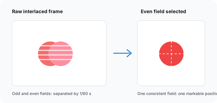
- Pause on the raw double image.
- Fields were captured 1/60 s apart.
- Select Video → Filters → New → Deinterlace.
- Use the Even field for this prepared route.
The two images are not two simultaneous ball positions.
BallDrop.mp4 demonstrates the method only. BallTossUp.mp4 is the one formal investigation.
Open the Practical Guide
Keep this Presentation available for whole-class checkpoints. Use the Guide for the detailed Tracker route.
Class resource: the Practical Guide becomes available from the lesson page after your teacher releases it to your class.
Checkpoint 1 | Audit the Setup
Do not start tracking until all five pass
- Even-field Deinterlace
- Frames 13–40; step size 1
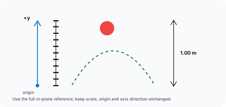
- Full white reference = 1.00 m
- Declared origin; upward-positive y
- One stated physical point on the ball
Checkpoint 2 | Track One Physical Point
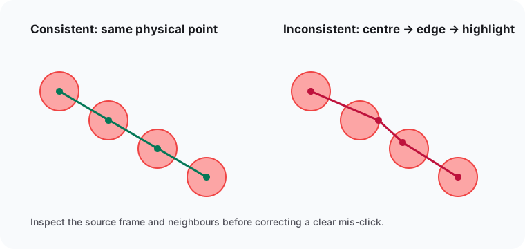
28 consecutive digital marks
Use every frame from 13 to 40. The five report rows are audit checkpoints, not the dataset.
Inspect frame → compare neighbours → retain or correct with a reason.
Do not delete every point that lies away from a fitted line.
Checkpoint 3 | Read the Evidence
Position–time
- Gradient decreases during ascent.
- Gradient is zero at the highest point.
- Gradient becomes negative during descent.
Velocity–time
- changes positive → zero → negative.
- The gradient remains negative at the zero crossing.
- Numerical differentiation amplifies point-placement variation.
L03 retains the systematic translation between motion graphs; here, use only the evidence needed to test the model.
Test the Constant-Acceleration Model
Measured acceleration
Fit the reliable velocity–time interval and compare the gradient with .
One consistent-start SUVAT check
Using SUVAT does not prove acceleration is constant.
Make a Qualified Model Decision
- State the fitted interval and signed acceleration.
- Compare with downward free-fall acceleration.
- Cite one supporting graph pattern.
- Identify one limitation tied to this evidence.
- Rank one improvement by likely impact.
Decide whether constant acceleration is supported within the resolution of the data.
Avoid a generic list of “human error”; explain the causal effect on this dataset.
Exit | Bridge to L03
How can while ?
Which feature of your position–time or velocity–time evidence should be interpreted more systematically next?
Complete the Post-practical Analysis in the same individual report. There is no separate Homework artifact.