A1 L03-1 | Reading and Calculating from Motion Graphs

Opening

Read the Graph

Position-Time Graphs

Velocity-Time Graphs

Acceleration-Time Graphs

Synthesis

IB Physics A.1 Kinematics | Lesson 3.1 | SL/HL

Reading and Calculating from Motion Graphs

Guiding question: Which graph operation reveals the physical quantity we need?

Learning Objectives and Success Criteria

Read

  • identify ordinate, gradient, signed area and interval
  • preserve direction through signs and units

Calculate

  • average and instantaneous velocity
  • acceleration, displacement and distance
  • change in velocity and final velocity

P01 Retrieval | Two Graphs, One Motion
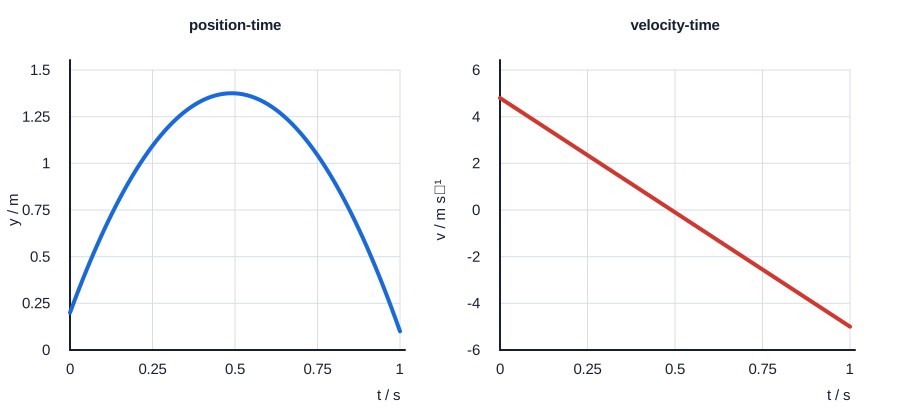
Position-time and velocity-time graphs for the same vertical toss.
Project-created graph; every calculation grid interval is labelled.

Figure 1 shows project-created graphs representing the vertical motion of a tossed ball. Upward is positive.

The graphs are an idealized backup representation of the pattern observed in A1 P01, not measured student data.

  1. (a) Identify the feature of the position-time graph that represents instantaneous velocity.
  2. (b) Explain why a curved position-time graph and an approximately straight velocity-time graph can describe the same motion.
  3. (c) State what the approximately constant negative gradient of the velocity-time graph indicates.
Reveal Q1 (1)

The tangent gradient at the chosen instant.

Velocity is the local rate of change of position, so it is represented by a tangent gradient.

Reveal Q1 (2)

The tangent gradient of the position-time graph changes continuously. Those instantaneous gradient values are the plotted velocity values, and they decrease approximately linearly with time.

The position graph is curved because its gradient is changing. The velocity graph records those changing gradients; a straight velocity-time graph means that the velocity changes by approximately equal amounts in equal time intervals.

Reveal Q1 (3)

Approximately constant negative acceleration.

Acceleration is the gradient of a velocity-time graph. A constant negative gradient therefore represents approximately constant negative acceleration.

A Motion Graph Is Not a Path Picture

Horizontal axis

Time advances from left to right. The graph records how one motion quantity changes with time.

Do not trace a route

A rising line does not mean the object travels uphill. Read the labelled axes first.

The Graph-Reading Contract

1 | Locate

Identify axes, units, instant or interval.

2 | Select

Ordinate, gradient or signed area?

3 | Interpret

Keep the sign, unit and any required initial value.

Say the operation before touching the numbers.

Operation Selection Check

For each requested quantity, state whether it is obtained by reading an ordinate, calculating a gradient, or calculating a signed area.

Use only one of: ordinate, gradient, signed area.

  1. (a) State the operation used to determine acceleration from a velocity-time graph.
  2. (b) State the operation used to determine displacement from a velocity-time graph.
  3. (c) State the operation used to determine change in velocity from an acceleration-time graph.
Reveal Q1 (1)

Gradient.

Acceleration is the rate of change of velocity, so it is the velocity-time gradient.

Reveal Q1 (2)

Signed area.

Velocity multiplied by time has unit metres, so the algebraic area is displacement.

Reveal Q1 (3)

Signed area.

Acceleration multiplied by time has unit metres per second, so the algebraic area is change in velocity.

Position-Time Graph | Ordinate and Gradient

Ordinate

The vertical coordinate gives position.

x=x(t)

Gradient

The gradient of a position-time graph gives velocity.

v=ΔxΔt

Chord Gradient | Average Velocity

Across a finite interval, average velocity is the average rate of change of position.

v¯=x2-x1t2-t1

Use the two interval endpoints and preserve the sign.

Tangent Gradient | Instantaneous Velocity

Ideal graph

The tangent gradient at one point gives the exact instantaneous velocity of the mathematical model.

Measured data

A local fit or a sufficiently short interval provides an estimate.

A chord across the whole graph is not generally instantaneous velocity.

Position Gradient Check | Chord and Tangent
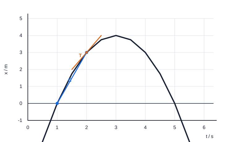
Position-time graph with a chord and a tangent.
Project-created graph; every calculation grid interval is labelled.

Figure 1 is a project-created position-time graph for an inspection cart. The curve follows x=4-(t-3)2, with x in metres and t in seconds.

Chord C joins (1.0s,0m) to (2.0s,3.0m). Tangent T touches the curve at t=2.0s and passes through (1.5s,2.0m) and (2.5s,4.0m).

  1. (a) Determine the average velocity from 1.0s to 2.0s using chord C.
  2. (b) Determine the instantaneous velocity at 2.0s using tangent T.
Reveal Q2 (1)

+3.0ms-1.

v¯=3.0-02.0-1.0=+3.0ms-1.

Reveal Q2 (2)

+2.0ms-1.

v=4.0-2.02.5-1.5=+2.0ms-1.

Zero Ordinate Is Not Zero Gradient

Position-time graph with a chord and a tangent.
Project-created graph; every calculation grid interval is labelled.

Figure 1 is a project-created position-time graph for an inspection cart. The curve follows x=4-(t-3)2, with x in metres and t in seconds.

Chord C joins (1.0s,0m) to (2.0s,3.0m). Tangent T touches the curve at t=2.0s and passes through (1.5s,2.0m) and (2.5s,4.0m).

  1. (a) At t=1.0s, the cart has x=0. Explain why its velocity is not zero.
  2. (b) At t=3.0s, the graph has a horizontal tangent. State the velocity and explain what happens to the direction of motion immediately after this instant.
Reveal Q3 (1)

Position is zero, but the tangent gradient is positive and non-zero.

The ordinate gives position, while velocity is the tangent gradient. The curve crosses x=0 with a positive slope.

Reveal Q3 (2)

v=0. The tangent gradient changes from positive to negative, so the cart reverses direction.

A horizontal tangent has zero gradient, so v=0. Before the maximum the gradient is positive; after the maximum it is negative.

Velocity-Time Graph | Gradient Gives Acceleration
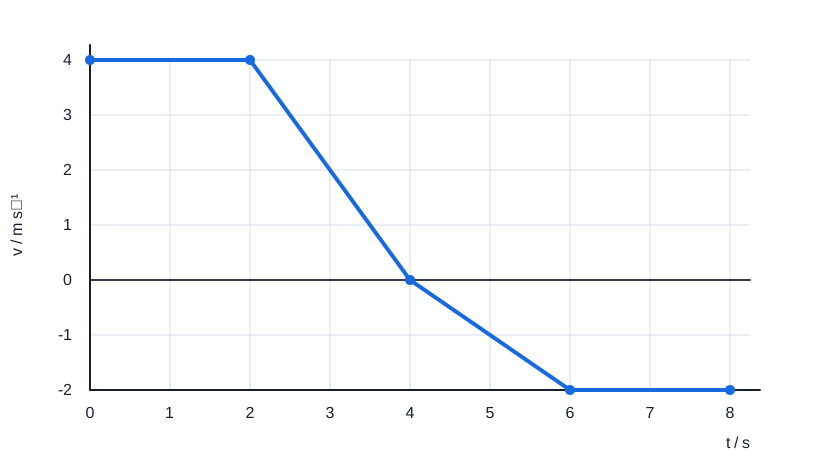
Piecewise velocity-time graph with positive and negative regions.
Project-created graph; every calculation grid interval is labelled.

Figure 1 shows a project-created velocity-time graph for a delivery drone moving along a straight rail. Positive velocity is toward the dispatch point.

Treat every straight segment as exact.

  1. (a) State the velocity at t=1.0s.
  2. (b) Determine the acceleration from t=2.0s to t=4.0s.
  3. (c) From t=4.0s to t=6.0s, state whether the drone is speeding up or slowing down. Explain using the signs of velocity and acceleration.
Reveal Q4 (1)

+4.0ms-1.

Read the ordinate directly: v=+4.0ms-1.

Reveal Q4 (2)

-2.0ms-2.

a=0-4.04.0-2.0=-2.0ms-2.

Reveal Q4 (3)

Speeding up. Both velocity and acceleration are negative.

After t=4.0s, the velocity is negative and becomes more negative, so the speed increases.

Velocity-Time Graph | Signed Area Gives Displacement

The signed area between a velocity-time graph and the time axis gives displacement.

Δx=signed area under the v-t graph

Use rectangles, triangles and trapezoids.

Displacement and Distance Use Area Differently

Displacement

Δx=A++A-

Add signed areas; the region below the time axis is negative.

Distance

d=|A+|+|A-|

Split at every zero crossing, then add magnitudes.

Velocity Area Check | Displacement versus Distance

Piecewise velocity-time graph with positive and negative regions.
Project-created graph; every calculation grid interval is labelled.

Figure 1 shows a project-created velocity-time graph for a delivery drone moving along a straight rail. Positive velocity is toward the dispatch point.

Treat every straight segment as exact.

  1. (a) Determine the displacement from t=0 to t=8.0s.
  2. (b) Determine the total distance travelled from t=0 to t=8.0s.
  3. (c) Explain why the displacement and distance answers are different.
Reveal Q5 (1)

+6.0m.

The positive areas are 8+4=12m. The negative areas are -2-4=-6m. Therefore
Δx=12-6=+6.0m.

Reveal Q5 (2)

18m.

d=8+4+2+4=18m.

Reveal Q5 (3)

Displacement uses signed area, whereas distance adds the magnitudes of all areas.

The negative-velocity intervals reduce signed displacement but still contribute positively to path length.

Acceleration-Time Graph | Signed Area Gives Change in Velocity

The signed area under an acceleration-time graph gives the change in velocity.

Δv=signed area under the a-t graph

The area gives a change, not automatically the final velocity.

Add the Initial Velocity

Area result

Δv=v-v0

Reconstruct the final value

v=v0+Δv

Two objects can share the same acceleration graph and still have different velocities.

Acceleration Area Check | Change and Final Value
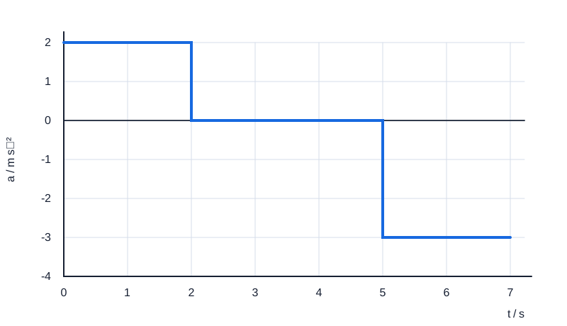
Piecewise acceleration-time graph.
Project-created graph; every calculation grid interval is labelled.

Figure 1 shows a project-created acceleration-time graph for a research sled. At t=0, its velocity is v0=-1.0ms-1.

Treat each horizontal section as exact.

  1. (a) State the acceleration at t=1.0s.
  2. (b) Determine the change in velocity from t=0 to t=7.0s.
  3. (c) Determine the velocity at t=7.0s.
  4. (d) Explain why the same acceleration-time graph could describe an object with a different final velocity.
Reveal Q6 (1)

+2.0ms-2.

Read the ordinate directly: a=+2.0ms-2.

Reveal Q6 (2)

Δv=-2.0ms-1.

Δv=(+2.0)(2.0)+(0)(3.0)+(-3.0)(2.0)=-2.0ms-1.

Reveal Q6 (3)

-3.0ms-1.

v=v0+Δv=-1.0-2.0=-3.0ms-1.

Reveal Q6 (4)

The acceleration-time area fixes only the change in velocity. A different initial velocity gives a different final velocity.

Every initial velocity is shifted by the same calculated Δv. The area does not specify v0.

Units Reveal the Graph Operation

x–t gradient

ms=ms-1

velocity

v–t gradient

ms-1s=ms-2

acceleration

v–t area

ms-1×s=m

displacement

a–t area

ms-2×s=ms-1

change in velocity

Mixed Checkpoint | Select Before Calculating
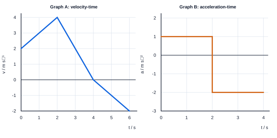
Velocity-time and acceleration-time graphs for two motion models.
Project-created graph; every calculation grid interval is labelled.

Figure 1 contains two independent, project-created motion graphs for an autonomous cart.

For graph B, the initial velocity is v0=+3.0ms-1.

  1. (a) From graph A, state the velocity at t=2.0s.
  2. (b) From graph A, determine the acceleration from t=2.0s to t=4.0s.
  3. (c) From graph B, determine the change in velocity from t=0 to t=4.0s.
  4. (d) Use the stated initial velocity to determine the final velocity for graph B.
Reveal Q7 (1)

+4.0ms-1.

Read the ordinate at 2.0s.

Reveal Q7 (2)

-2.0ms-2.

a=0-4.04.0-2.0=-2.0ms-2.

Reveal Q7 (3)

Δv=-2.0ms-1.

Δv=(+1.0)(2.0)+(-2.0)(2.0)=-2.0ms-1.

Reveal Q7 (4)

+1.0ms-1.

v=v0+Δv=3.0-2.0=+1.0ms-1.

Common Misconceptions to Eliminate

Graph shape

Do not treat a graph as the object's route.

Zero values

Zero ordinate and zero gradient are different statements.

Area sign

Below-axis velocity contributes negative displacement but positive distance.

Initial value

Acceleration-time area is change in velocity; add the initial velocity.

Exit Bridge | Predict One Related-Graph Feature

Use ordinate-gradient-area relationships to predict one feature of a related graph.

Do not sketch a complete graph.

  1. (a) A position-time graph is a straight line with constant positive gradient. Predict the corresponding velocity-time graph feature.
  2. (b) A velocity-time graph is horizontal above the time axis. Predict the corresponding acceleration-time graph feature.
Reveal Q1 (1)

A horizontal velocity-time line at a constant positive velocity.

The position-time gradient is velocity. A constant positive gradient therefore gives constant positive velocity.

Reveal Q1 (2)

A horizontal acceleration-time line at a=0.

The velocity-time gradient is acceleration. A horizontal velocity-time graph has zero gradient.

1 / 22